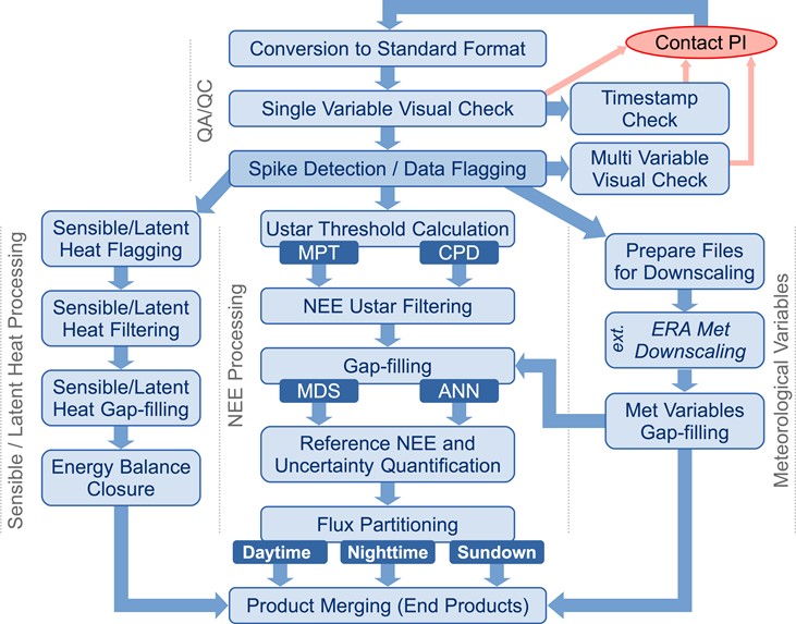
A unique contribution of FLUXNET is its assembly and delivery of uniform, harmonized, and well-vetted flux products for a global network of sites, for use by modeling, remote sensing, and data synthesis communities, and shared among regional research networks. This product involves producing gap-filled data sets that can be integrated or averaged on daily to annual time scales, producing estimates of uncertainty about the fluxes, and partitioning net carbon fluxes into photosynthetic and respiratory components. Below we describe the key steps in producing this database.
Data collected by local tower teams are first submitted to the data archives that are typically hosted by the regional networks. The data are pre-screened and formatted based on the regional network data protocols. After the data are posted by the regional networks, the data then enter the Fluxdata processing pipeline with the consent from the tower investigators. The data are checked for obvious problems, like errors in time stamps, unexplained jumps in the variables due to sensor malfunction, spikes, values out of range, and errors in units; this is accomplished by visualization and producing statistical metrics. Detailed checks are also performed on variables that directly affect the results of the processing. These secondary checks take into account multiple temporal scales and conditions specific to each site and equipment deployed. At this initial stage, the Fluxdata processing team works with investigators to correct the identified data problems and generate a new version of the data set.
After data pass the pre-screening criteria, data files are assigned names based on a standard convention that describes the site name and year. Data columns within the files are checked for having proper names, labels, and units. These data files, which contain gaps and are otherwise unchanged from what was submitted by the data producers, are the first level of data product. The next data processing step subjects the data to quality flagging, filtering, and gap-filling. We look for spikes, extreme outliers and non-physical values in the data, and these data are flagged. In a subsequent step, data are filtered and bad data are replaced or filled with highly vetted gap-filling methods. The current data release, produced by a Fluxdata team that is a confederation of resources from across the regional networks such as ICOS and AmeriFlux, uses the marginal distribution sampling (MDS) method of Reichstein et al (2005) and Artificial Neural Networks, which proved to be two of the best among many gap-filling methods tested (Moffat et al., 2007). We find it to be preferable to fill gaps with the empirical MDS method, than to fill gaps with non-linear multi-variate models (Falge et al., 2001).
Net carbon fluxes will be partitioned into Gross Primary Production (GPP) and Total Ecosystem Respiration (TER) using two different and alternative approaches: the first based on the extrapolation of night-time data based on temperature (Reichstein et al., 2005) and the second based on light-response curve optimization using day-time measurements (Lasslop et al., 2010). The two methods give independent partitioning of GPP and TER that can be used also as uncertainty indicators. A third partitioning method (van Gorsel et al. 2009) is being tested and applied to sites where conditions allow. This method uses the respiration levels at sunset to estimate nighttime respiration.
The Figure below highlights the ICOS-AmeriFlux-FLUXNET data pipeline.